Orientation Discrimination: Lesson 4

SPATIAL & TEMPORAL CONTEXTUAL EFFECTS

This lesson makes the basic orientation discrimination task more elaborate by displaying a surrounding stimulus to investigate both spatial and temporal contextual effects.

First, duplicate the original experiment, rename the copy Orientation Discrimination 4, and move it to the top of the Designer table. Reveal its whole hierarchy by option-clicking on its arrow.

Step 1: Creating a Center-Surround Stimulus

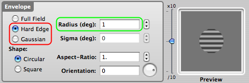
Rename the Gabor stimulus to Center. Edit the Center stimulus properties to change the envelope shape from Gaussian to Hard Edge. Set its radius to 1 deg.

Click on the OK button to validate the changes.

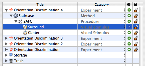
Create a new stimulus just above the Center stimulus. Set its category to Visual Stimulus and name it Surround.

Edit the properties of the Surround stimulus.

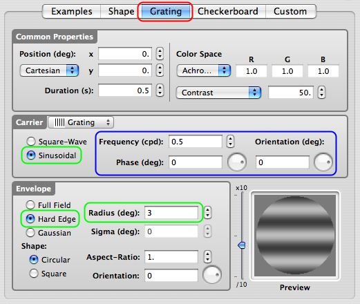
Select the Grating tab. Set the carrier type to Grating with a Sinusoidal profile.

Set the envelope to Hard Edge and its radius to 3 deg (this must be larger than the radius used for the Center stimulus).

The spatial frequency, phase, and orientation of the Surround carrier are the properties that are likely to modulate the contextual effects on the orientation discrimination for the Center stimulus. For example, the cross-orientation effect could be investigated by leaving the Surround orientation at 0 deg if the Center orientation varies close to 90 deg.

Click on the OK button to validate the changes.

Step 2: Adding a Timeline Event

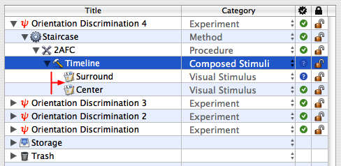
Create a Timeline event inside the 2AFC event as you did in Orientation Discrimination Lesson 2. Move the two stimuli (Surround and Center) inside the Timeline, so they appear indented, as illustrated; they can be selected together and then dragged & dropped onto the Timeline.

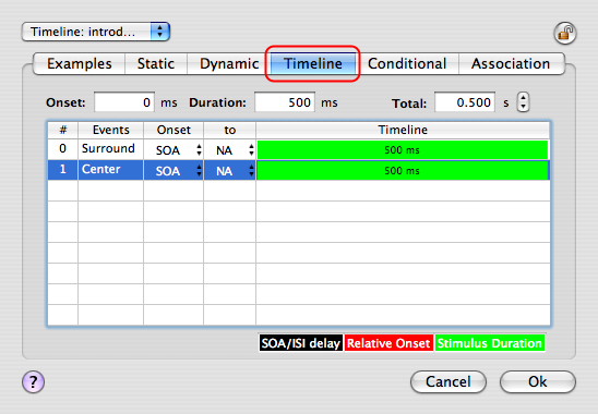
Edit the properties of the Timeline event.

Select the Timeline tab.

The next step is to reduce the duration of the Center stimulus and introduce an SOA (stimulus onset asynchrony) between the Surround and the Center.

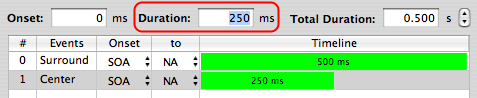
Select the Center entry in the timeline table and change its duration to 250 ms.

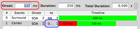
Set the Onset of the Center stimulus to 125 ms (this is automatically rounded to the frame duration), its Onset column to SOA, and its to column to 0: Surround.

The Center timeline is now split in two, with the red zone corresponding to the SOA period relative to the Surround onset.

Click on the OK button to validate the changes.

Step 3: Blending the Center & Surround

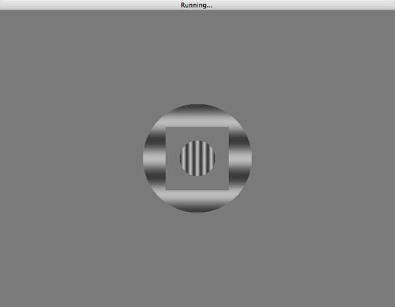
If you ran the experiment as it is defined now, the presentation would look as shown above: a Center stimulus inscribed in a gray square superimposed onto the Surround stimulus. This is because stimuli are generated on an empty square array regardless of the geometry of their content.

The gray surrounding in the Center stimulus should be made transparent so the Surround stimulus is only occluded by the circular part of the central grating.

The gray surrounding of the Center stimulus can be made transparent using OpenGL blending.

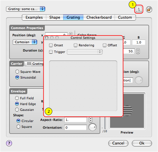
To specify the blending options, edit the Center properties and click on the small switch icon (1) in the top right-hand corner of the panel. This opens a palette entitled Control Settings (2) which provides further settings for various aspects of the stimuli presentation.

This palette allows you to fine-tune how stimuli are rendered by the OpenGL engine during onset, offset, and rendering times. Initially, this palette displays an empty box with unchecked buttons above it.

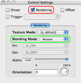
To modify the way the stimulus is composed with the previously displayed stimuli, check the Rendering box.

The Rendering settings consist of the following:

- Texture mode
- Blending mode that specifies the composing operation (Replace by default)
- Source (the current stimulus) and destination (the already drawn stimuli) factors
- Transparency level
- Orientation to be applied

Note that all these operations are performed by the graphics hardware and are consequently extremely fast.

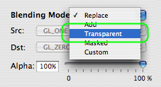
Select the Transparent option from the blending mode pop-up menu.

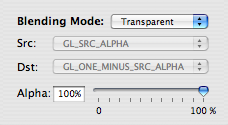
The source and destination factors are automatically set to values that implement the transparency for the gray part of the stimulus.

Click on the OK button to validate the changes (this also closes the Control Settings palette).

Check & run the Experiment!

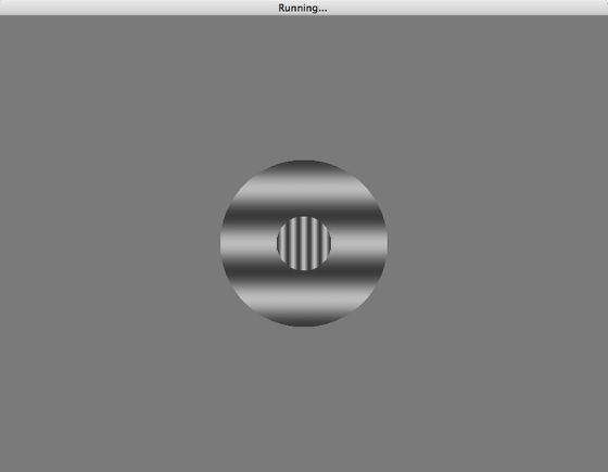
Shown above is what is produced with the OpenGL transparent blending set for the Center stimulus.

Conclusion

In this lesson you learned how to create an SOA between stimuli and properly combine stimuli using OpenGL blending capabilities.

In the last lesson, you will learn how to add motion & dynamics through the use of a 1st-order drifting Gabor (Lesson 5).