


Basic stimuli presented in the "Visual Stimuli" section can be repeated and pasted across space and time to produce multi-element stimuli.
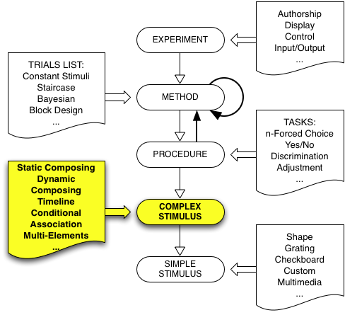
Psykinematix offers the possibility of creating
multi-element stimuli that consist of either dynamic (RDK) or static (MEF and
SSS) element fields:
Random-Dot Kinematogram (RDK)
Multi-Element Field (MEF)
Sampled-Shape Stimulus (SSS)
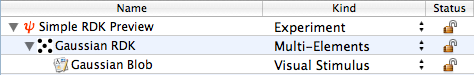
To create a Multi-Element Stimulus (as illustrated in the example below), create a new group event in the "Experiment Designer" window, set its category to "Multi-Elements", and display its properties by clicking on the "Info" icon (or press Apple-I). Once a RDK or MEF stimulus has been selected, changing it by clicking on other tabs is disabled unless the Control key is pressed simultaneously. This is to prevent accidental changes because stimulus settings are then reset to default.
For each type of multi-element stimuli listed above, it is possible to create a list of different visual elements, hence producing heterogeneous multi-element stimuli commonly used in visual search, spatial integration, etc. The spatial spread of the elements is indicated by the preview in the bottom right-hand corner of the Area or Grid Properties.
Example:
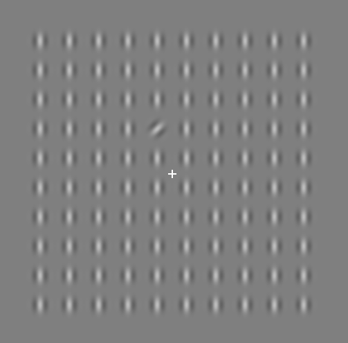
Random-dot kinematogram (RDK) is a special class of visual stimuli for investigating how local motion is integrated into global motion. Such a stimulus consists of a population of similar elements that move either coherently or randomly. These elements were originally only small dots, but Psykinematix is flexible enough to allow any type of visual stimulus to be used so that several types of elements can be combined to produce heterogeneous RDKs as illustrated below.
Limited lifetime RDK |
Rotating and expanding RDKs |
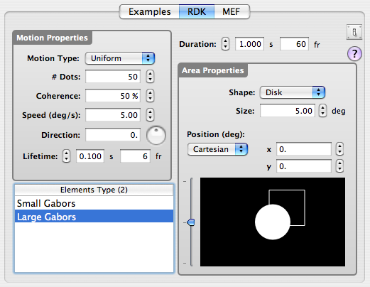
As illustrated in the panel above, the RDK properties are of two types, those describing the motion properties (on the left) and those describing the spatial properties of the motion area (on the right):
-
The motion properties consist of:
- the motion type (uniform, radial, or angular),
- the number of dots,
- the coherence level in percent (i.e. proportion of dots that move coherently),
- the speed of each individual dot in deg/s,
- the motion direction of coherent dots,
- the lifetime of each element expressed either in seconds or number of frames (use 'inf', 'infinity' or '∞' for infinite lifetime). Dots with a limited lifetime are repositioned at random locations in their motion area after their lifetime expires. Note that the temporal phase for limited lifetime elements is chosen randomly at onset time,
Note that the motion direction is described differently from the motion type:
- For uniform motion, the direction is an angle expressed in degrees (0 deg for left to right motion, 90 deg for bottom to top motion);
- For radial motion, the direction is selected through a pop-up menu as either inward (periphery to center) or outward (center to periphery),
- For angular motion, the selectable directions are clockwise or anticlockwise.
Note that when using a mathematical expression or a variable to specify the direction for radial or angular motion, a negative direction indicates an inward or anticlockwise motion, and a positive direction indicates an outward or clockwise motion. Both speed and direction can also be specified for individual dots by using an expression between { } symbols: for example, the expression '{0:180}' for the direction indicates that the direction for individual dots is randomly and uniformly chosen between 0 and 180 degrees. Without the { } symbols, the expression indicates that the same random direction applies to all dots.
-
The area properties specify the spatial field on which the moving dots are drawn, and consist of:
- the surface shape (square or disk),
- its size (side for square, diameter for disk),
- its position in the visual field (expressed either in Cartesian or polar coordinates).
The drawing area at the bottom depicts the shape and location of the area used by each type of dot (filled area for currently selected types, outline for unselected types). Control-clicking inside this area displays a contextual pop-up menu that provides an OpenGL preview that can be optionally exported to a Quicktime movie.
-
The duration of the motion presentation is specified above the area properties either in seconds or by the number of frames.
- The list of element types that compose the RDK is presented
in the table at the bottom-left corner of this panel. Each element type can
have its own motion and area properties.
Note that the element types cannot be added, removed, or reordered directly from this panel. These actions should be performed through the "Experiment Designer" window. However, the motion or area properties can be assigned to a group of entries by selecting them from the list and changing their properties.
RDK stimuli can appear as a node inside these categories:
- Experiment
- Method
- Procedure
- Composed Stimuli (except Static)
Several examples of RDK stimuli are available in "Demos, Examples & Tutorials" in the Storage area of the Designer Panel (Multi-Elements subsection in the Stimuli section).
Multi-element fields (MEFs) are static or dynamic versions of RDKs where the position of each element is constrained to a polar or Cartesian grid. This type of stimulus category is useful for investigating visual searches, pop-out effects, etc. The grid can be populated with several types of non-overlapping elements as illustrated by the following examples:
 Oblique target embedded in a field of vertical distracters |
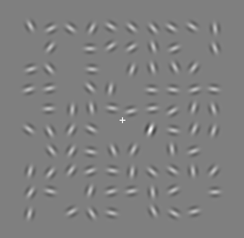 High contrast target embedded in a field of low contrast distracters |
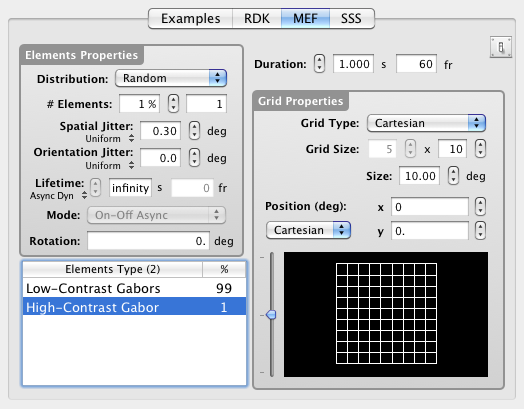
As illustrated in the panel above, the MEF properties are of two types, those describing the element sets (on the left) and those describing the grid (on the right):
-
The properties of each element set consist of:
- the type of spatial distribution ('Random' or 'Glass Patterns'):
- with the 'Random' distribution there is no specific constraint applied on the field except that the orientation and spatial jitters are applied independently of the element absolute position and rotation,
- with the 'Glass Patterns' distribution there is a specific constraint applied on the element orientation once the jittered position has been defined: its orientation is set so it is tangent to a circle centered of the field and passing through the element. The rotation and orientation jitter are then applied relative to this reference orientation.
- the contribution of the specified set expressed either as the percentage or number of elements (note that the total number of elements can be fewer than the grid permits thus leaving some "holes" in the grid),
- the spatial and orientation jitters (in degree) to be applied to each element of the set; the distribution type (uniform or Gaussian) can be also specified ([-jitter,+jitter] range for uniform, jitter standard deviation for Gaussian),
- the lifetime of each element expressed either in seconds or number of frames (use 'inf', 'infinity' or '∞' for infinite lifetime),
- the lifetime mode ('On-Off', 'Field Update' or 'Shuffle') that
specified what happens once the life-time of each element has expired
and whether this happens synchronously
or asynchronously (random relative phase) amongst the different
elements:
- in the 'On-Off' mode, the elements disappear for the same life-time duration before reappearing;
- in the 'Field Update' mode, the elements have their position and orientation reset based on the specified position and orientation jitters (but at the same grid position!);
- in the 'Shuffle' mode, the elements have their position and orientation reset based on the specified position and orientation jitters, but at a possibly different grid position based on availability at the reshuffling time (based on number of empty locations and other elements being reshuffled). Note that the rotation parameter (see below) is not supported in the 'Shuffle' mode with the 'Random' distribution (see above).
- the rotation (in deg) to be applied onto each element of the set. When put between { }, the rotation expression is evaluated on an element basis: for example, the expression '{90*round(rnd)}' would specify a rotation of 0 or 90 deg on a random basis. This rotation can even be specified as function of the element position relative to the grid center: in such expression, variables x, y, r, and theta between { } indicate the Cartesian and polar coordinates of each element before the position and orientation jitters are applied. For example, to create concentrically-aligned Gabor elements, set the element rotation to '{theta}' if the element is defined as a vertical Gabor. Note that the rotation parameter is not supported in the 'Shuffle' mode with the 'Random' distribution (see above).
-
The grid properties specify:
- the geometry (Cartesian or polar),
- the spatial field in degree,
- the number of samples (i.e. maximum number of elements) on the grid,
- its position in the visual field (expressed either in Cartesian or polar coordinates). Mathematical expressions can be used to specify the Cartesian or polar coordinates. Note that the x-axis position supports the monocular and disparity formats (see the "Visual Stimuli" section for more details).
The drawing area at the bottom depicts the shape and location of the grid. Control-clicking inside this area displays a contextual pop-up menu that provides an OpenGL preview that can be optionally exported to a Quicktime movie.
-
The duration of the field presentation is specified above the grid properties either in seconds or by the number of frames.
It is important to note that the element types cannot be added, removed, or reordered directly from this panel. These actions should be performed through the "Experiment Designer" window. However, the distribution properties inside the grid can be assigned to a group of entries by selecting them from the list, and changing their properties.
Note also that the seed used for the random distribution of the different elements in the MEF grid can be explicitly specified by clicking on the Distribution label as illustrated below:
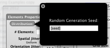
By default, the 'seed' field is empty and then considered as unspecified: in this case the generation of each MEF distribution is random and uncorrelated from one instance to another one. If the 'seed' value is specified through an integer value or a variable (whose value can be itself randomly generated), then the same distribution is generated with the same seed value. This is useful when one needs to generate the same distribution of elements like for example in dichoptic presentations (if using a variable, remember to use it with the $ prefix in subsequent MEF instances, eg. [$seed]).
Finally, MEF stimuli may embed dynamic elements as illustrated below:
Field of drifting Gabors |
Oscillating Elements |
MEF stimuli can appear as a node inside these categories:
- Experiment
- Method
- Procedure
- Composed Stimuli (except Static)
Several examples of MEF stimuli are available in "Demos, Examples & Tutorials" in the Storage area of the Designer Panel (Multi-Elements subsection in the Stimuli section).
Sampled-shape stimuli (SSS) are similar to multi-element fields (MEFs) except that their distribution is not constrained to a polar or Cartesian grid. Their spatial distribution can be anything either structured (eg, along a curve) or completely random. This type of stimulus category is useful for investigating shape perception using well controlled discrete spatial elements. Several types of elements can be mixed and their overlapping can be prevented if needed as illustrated by the following examples:
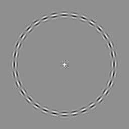 Gabors along a circular curve |
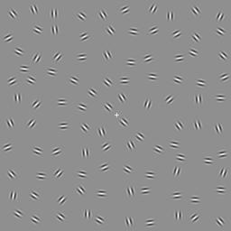 Contour made of collinear Gabors embedded in a field of randomly oriented Gabors |

As illustrated in the panel above, the SSS properties are of two types, those describing the spatial properties of the element sets (on the left) and those describing their spatial distribution (on the right):
-
The properties of each element set consist of:
- the type of spatial distribution (analytical by default):
- with the 'analytical' distribution the elements position is described analytically through their Cartesian or polar coordinates, and elements of different types are pasted independently and may or not overlap (see column entitled 'deg' below),
- similarly with the 'analytical with mixing' distribution the elements position is described analytically through their Cartesian or polar coordinates, but the elements of different types are not anymore pasted independently: those with location described by the same expressions are combined together and randomly mixed so they do not overlap (this is similar to the MEF distribution without being restricted to a polar or Cartesian grid).
- the number of elements (note that the number of displayed elements can be fewer if overlap between elements of different sets is prohibited),
- the spatial and orientation jitters (in degree) to be applied to each element of the set; the distribution type (uniform or Gaussian) can be also specified ([-jitter,+jitter] range for uniform, jitter standard deviation for Gaussian),
- the lifetime of each element expressed either in seconds or number of frames (use 'inf', 'infinity' or '∞' for infinite lifetime),
- the lifetime mode ('On-Off' or 'Field Update') that
specified what happens once the life-time of each element has expired and whether this happens synchronously
or asynchronously (random relative phase) amongst the different elements:
- in the 'On-Off' mode, the elements disappear for the same life-time duration before reappearing;
- in the 'Field Update', the elements have their position and orientation reset based on the specified position and orientation jitters (but at the same grid position!).
- the rotation (in deg) to be applied onto each element of the set. When put between { }, the rotation expression is evaluated on an element basis: for example, the expression '{90*round(rnd)}' would specify a rotation of 0 or 90 deg on a random basis. This rotation can even be specified as function of the element position relative to the grid center: in such expression, variables x, y, r, and theta between { } indicate the Cartesian and polar coordinates of each element before the position and orientation jitters are applied. For example, to create concentrically-aligned Gabor elements, set the element rotation to '{theta}' if the element is defined as a vertical Gabor. The rotation can also be specified as a function of the element index i (from 0 to elements number minus 1) or the curvature (local orientation) k along the curve defined by the spatial distribution (see below). For example, to create collinear Gabors along a curve, set the element rotation to '{k}' if the element is defined as a horizontal Gabor.
- the column entitled 'deg' in the table with its associated stepper
control indicates the minimum distance below which overlap between
elements of different sets is prohibited: setting this value to
0 deg indicates that the set does not preclude overlap with other
sets. When overlap is detected the displayed element is coming
from the set with the highest priority that is the first one
listed in the table (the second set listed has the second highest
priority, and so on).
- the type of spatial distribution (analytical by default):
-
The distribution properties specify:
- the position of each element expressed either in Cartesian or polar coordinates (relative to its center defined below). The position should be a function of the element index i between { } or entirely between { } if the element index is not used because it is irrelevant to the position (otherwise the position is the same for all elements). The curvature along the curve defined by these ordered positions defines the variable k that can be used to specify a rotation for each element (see above).
- the 'center' position of the distribution in the visual field (expressed either in Cartesian or polar coordinates). Mathematical expressions can be used to specify the Cartesian or polar coordinates. Note that the x-axis position supports the monocular and disparity formats (see the "Visual Stimuli" section for more details).
The drawing area at the bottom depicts the spatial distribution of each set along with the rotation applied to each element. Control-clicking inside this area displays a contextual pop-up menu that provides an OpenGL preview that can be optionally exported to a Quicktime movie.
-
The duration of the field presentation is specified above the distribution properties either in seconds or by the number of frames.
Note that the element types cannot be added, removed, or reordered directly from this panel. These actions should be performed through the "Experiment Designer" window. However, the distribution properties inside the grid can be assigned to a group of entries by selecting them from the list, and changing their properties.
Finally, SSS stimuli may embed dynamic elements as illustrated below:
Interleaved Drifting Gabors |
Inward/Outward Drifting Gabors |
SSS stimuli can appear as a node inside these categories:
- Experiment
- Method
- Procedure
- Composed Stimuli (except Static)
Several examples of SSS stimuli are available in "Demos, Examples & Tutorials" in the Storage area of the Designer Panel (Multi-Elements subsection in the Stimuli section).