Import, Plot, Fit, and Export Data

Introduction

To start, click the Plotter icon in the toolbar. This opens the Plotter panel as shown below.

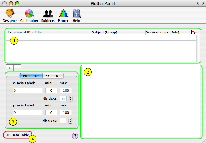
The Plotter panel presents:

1) a table that lists, using a hierarchical structure, the results of the last performed sessions or imported sessions;

2) a graphing view where selected datasets are plotted;

3) a 'tab' panel that allows the customization of the plots (Properties), and fitting parameters for each data type (XY, RT, etc).

4) a small arrow in the bottom-left corner marked Data Table that can reveal a drawer containing the data attached to the current selection in table (1).

Step 1. Importing the Data

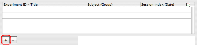
Table (1) usually contains the session results collected since the last launch of Psykinematix. To access results from previous sessions, you have to import them using the '+' button below the table (this can be also performed through the Import Session button present in the Subjects panel, see the Manage Subjects, Groups and Sessions tutorial).

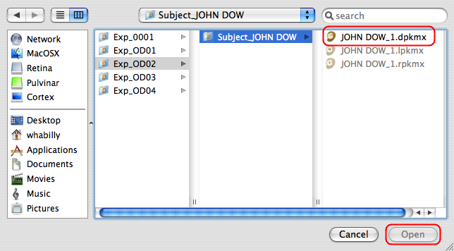
When clicking the '+' button, you are presented with a file selection panel that allows you to select which data file to import in the Plotter table. These files have a 'dpkmx' extension and are located in the folder where your session data are stored ('~/Desktop/MyExperiments' by default).

Select a data file and click the Open button.

Each new entry in the table provides a summary of the session information that consists of:

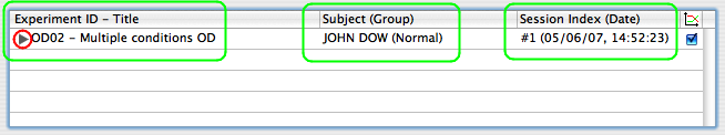
- Experiment ID and experiment title;
- Subject and group names;
- Session index and date.

This is the first level of the results hierarchy. Click the arrow in front of the session entry to reveal the next level.

The second level of the results hierarchy presents the datasets collected during the session for each experimental condition. Each entry of this level provides a summary of the dataset that consists of:

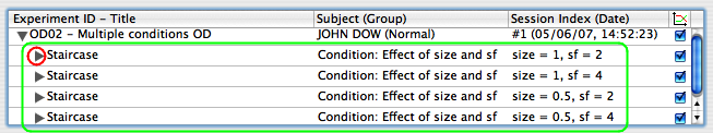
- Method name;
- Condition name;
- Parameters values.

Click the arrow in front of the datasets entry to reveal the next level.

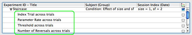
The third level of the results hierarchy presents the individual data collected during the session. The nature of the data is explicitly described by their title.

If you want to remove any data entry from the table (and at any level of the hierarchy), select it and click the '-' button. Note that the file that actually stores the data is nor deleted or modified. Data can be added again to the table at any time with the '+' button.

Step 2. Plotting the Data

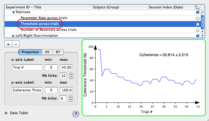
The selected data in the third level of the hierarchy described above is automatically plotted in the graphing view with the appropriate axis, labels and legends.

Depending on the nature of the plotted dataset, It is possible to customize its graphing properties.

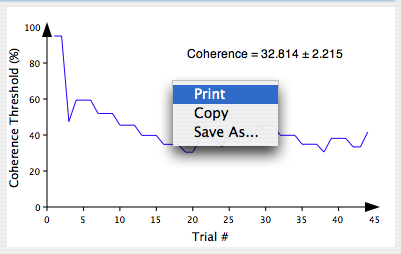
The graph can be either printed, copied or saved by control-clicking onto the graphing view. A copied graph can be pasted in any document that supports PDF. A saved graph is also in PDF format and can be edited in any application that supports the PDF format.

Step 3. Fitting the Data

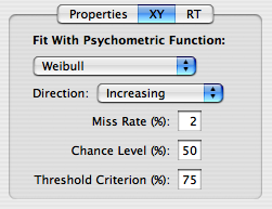
For methods that do not already perform some data analysis, their dataset can be fitted with a psychometric function selected in the XY or RT tab panel depending on the data type.

If appropriate data are plotted in the graphing view, changes made in the fitting parameters are automatically reflected in the graph.

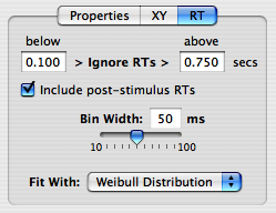
If reaction times are collected during a session, their distribution is represented as an histogram whose bin width can be specified here. The original RTs can be also filtered to remove too short or too long values before drawing and fitting the histogram. The histogram can be optionally fitted with a Weibull distribution. Post-stimulus RTs can be optionally included in both histogram and fit.

Step 4. Exporting the Data

Clicking the small arrow in the bottom-left corner reveals a drawer with a table representation of the data. The data presented in this table depends on the selection in the Session table (1).

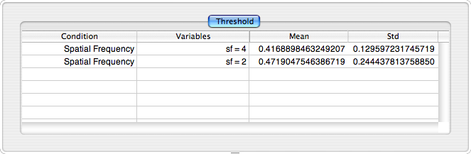
Selecting a Session entry (1st-level of the results hierarchy) shows a summary of the analysis performed on each dataset (typically thresholds and/or slopes as function of the experimental condition). The result type is indicated by the "tab" title: in this example some thresholds were measured (as mean and std) for two experimental conditions to look at the effect of spatial frequency.

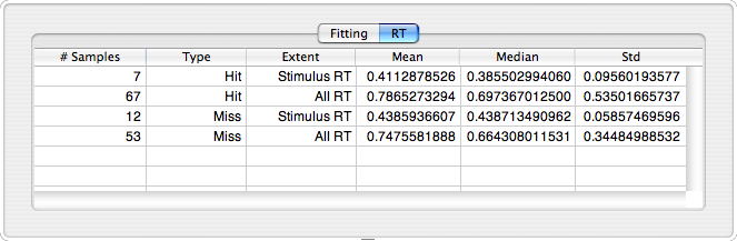
In this example, RTs were also collected and the statistics of their distribution reported as mean, median and std for each type of responses (hit & miss) including and excluding post-stimulus RTs ('All RT' and 'Stimulus RT' extent, respectively).

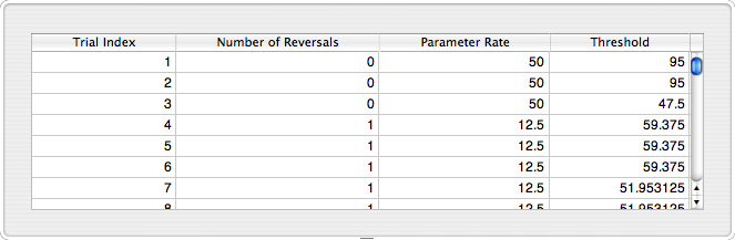
This is an example of data table obtained when selecting a datasets entry (2nd level of the results hierarchy): each data type collected during the session for a particular experimental condition appears as a column, with one row for each trial.

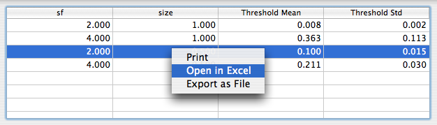
By control-clicking inside the table, presented data can be either printed, exported to a tabulated text file, or opened in Excel or Numbers applications for further analysis.

Conclusion

In this tutorial, you learned how to import and inspect previously collected session data, plot them with their fitting function, and export them under various forms.