
|
Visual Stimuli |
Visual stimuli are the most basic aspect of the experimental protocol, and often the most critical one as the choice of stimuli and of their parameters may define and limit the scope of your experiments. Psykinematix provides convenient tools to specify their spatial, temporal, and chromatic properties. Most stimuli properties can be specified with values, variables, or mathematical expressions.
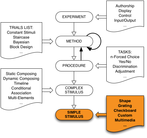
Psykinematix offers the possibility of creating a large variety of basic visual stimuli:
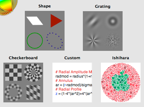
Shape Stimuli
Grating Stimuli
Checkerboard Stimuli
Custom Stimuli
Ishihara Stimuli
To create a Visual Stimulus, create a new single event in the "Experiment Designer" window, set its kind to "Visual Stimulus", and display its properties by clicking on the "Info" icon (or press ⌘I). Once a stimulus has been selected, changing it by clicking on other tabs is disabled unless the Control key is pressed simultaneously. This is to prevent accidental changes because stimulus settings are then reset to default.
The specification panel for each stimulus category is divided into 4 parts:
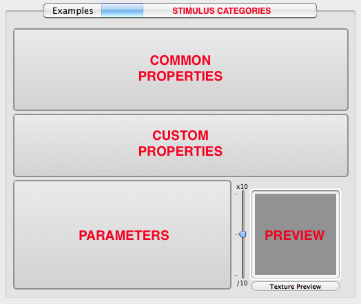
Common properties (top part of the panel) which consist of the:
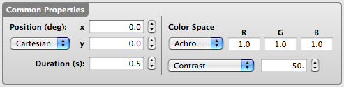
position of the stimulus center in degrees that can be specified in terms of Cartesian (x,y) or polar (r,theta) coordinates relative to the display center. For 2D rendering (single display) the x coordinate consists in a single expression. For Stereo or Anaglyph rendering (see Rendering Modes in Defaults Preferences), the x coordinate can take the following forms to specify whether it applies to the left or right display, to both displays or whether it also specifies a disparity value (always expressed in arcmin, positive for cross-disparity or 'in front' presentation, negative for uncrossed disparity or 'behind' presentation):
An additional option (Mouse-Driven) allows the stimulus to follow the mouse position (the x,y coordinates are then specified with the system-defined variables [XMOUSEDEG] and [YMOUSEDEG]).
stimulus duration in seconds.
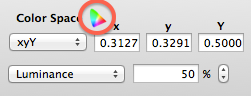
chromatic appearance of the stimulus in terms of color space (achromatic, RGB, LMS, XYZ, HSB, La*b*, xyY Yuv, L*u*v*), tri-stimulus values, modulation type (contrast, luminance or custom), and modulation strength (in %). Note that some color spaces can only specify luminance or contrast. By setting the modulation type to dark or light contrast/luminance, it is possible to specify two chromatic directions for the dark/negative and light/positive parts of the stimulus, respectively. Note that contrast refers to Michelson contrast (defined as [maxlum-minlum]/[maxlum+minlum] or Δlum/meanlum) along the specified chromatic vector (as a percentage relative to the maximum contrast obtained for the achromatic vector). A custom chromatic mode is also available to specify explicitly the trichromatic values on a pixel basis (this mode is only available for the Custom Stimulus category using the zr, zg, and zb output variables, and the modulation strength does not apply in this case).
Note that information about the luminance and color resolution expressed in bits and the minimum stepsize for contrast and luminance expressed in percent is available by clicking on the Color Space label as illustrated above.
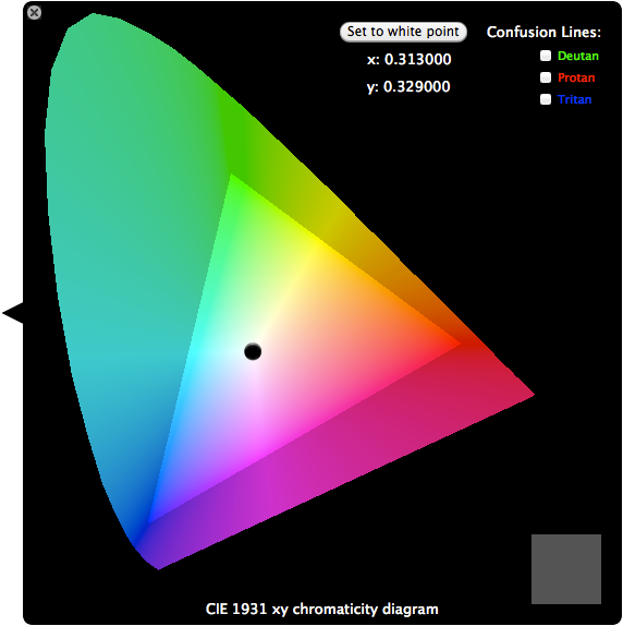
When specifying the stimulus luminance in the xyY or Yu'v' color space, it is possible to specify the chromatic coordinates using a CIE diagram available by clicking the small diagram icon as highlighted above. This diagram shows the gamut of the display used to present the stimulus and the coordinates selection is limited to the inside of this gamut triangle. The white cross shows the white point and the indicated chromatic coordinates are for the position of current marker (empty circle). To validate these coordinates for the stimulus, click inside the marker which then becomes filled. The protan, deutan and tritan confusion lines relative to the marker coordinates can be also added to this CIE diagram (with deutan, protan and tritan copunctal coordinates of (1.4,-0.4), (0.7635, 0.2365) and (0.1748, 0) respectively [Smith & Pokorny 2003]).
Custom properties (central part of the panel) that customize the shape or type of stimuli.
Parameters (bottom-left quadrant of the panel) common to all shapes or types of stimuli defined above.
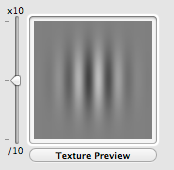
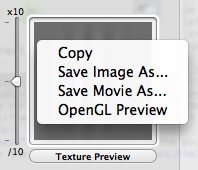
A preview (bottom-right quadrant of the panel) which is automatically updated with changes in parameter values. The preview details can be zoomed in and out using the slider on its left. In texture preview mode, by control-clicking inside the preview you can either copy the preview image, save it as an image file in TIFF format, save it as a movie, or preview it through the OpenGL rendering engine used during an actual experimental session. For custom stimuli the preview can display the stimulus either in the spatial or Fourier domain. The size of the OpenGL preview can be customized under the Defaults tab of the Preferences Panel.
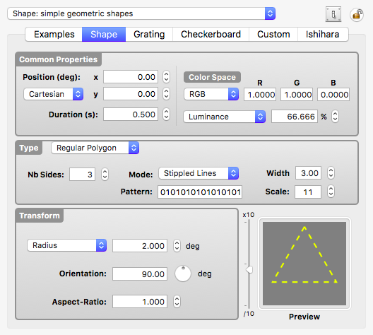
Shape stimuli consist of simple shapes based on regular polygons characterized by their number of sides: triangle, square, pentagon, hexagon, etc. Approximated circles are formed using a very large number of sides.
These shapes can be filled or delineated by either plain lines, stippled lines or points. The available thickness for the lines and points depends on the graphics board. Pattern and scale are only used by stippled lines. The chromaticity, luminance or contrast of the filling or of the border can be specified; however, for the contrast the color appearance depends on its sign.
Note that for the points to appear as circles, the blending mode in the rendering settings has to be set to Transparent (Src: GL_SRC_ALPHA, Dst: GL_ONE_MINUS_SRC_ALPHA). This blending mode also provides antialiasing for the line mode (and the fill mode if your graphics card still supports it).
The geometry of these shapes can be transformed by varying their size (through the radius between the center of the shape and its vertices), orientation, and aspect-ratio along the x-axis.
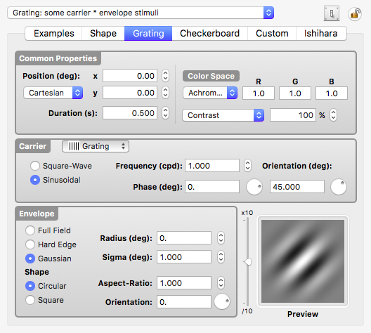
Grating stimuli consist of a carrier pattern modulated by an optional envelope. They can be either contrast-defined or luminance-defined.
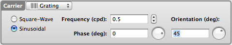
Carrier:
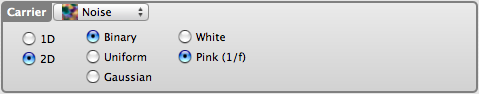
Several carrier types are available. The carrier type is selected through a pop-up menu:
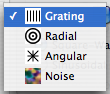
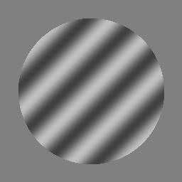
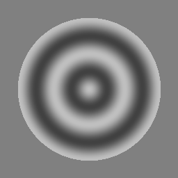
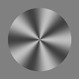
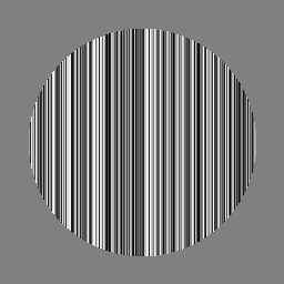
Grating, Radial, Angular carrier types only differ by the spatial dimension along which their luminance profile is modulated (x-axis, radius-axis, angular-axis). This luminance profile follows a square-wave or a sinusoidal modulation at a given spatial frequency, a phase, and an orientation (orientation is only valid for the Grating type).
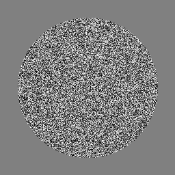
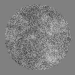
Noise carriers can either be 1D or 2D with a binary, uniform, or Gaussian distribution (based on contrast range) and a white or pink (1/f) spectral distribution in the Fourier domain.
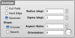
Envelope:
The role of the envelope is to limit the visibility of the carrier. Its size, shape, orientation, and aspect-ratio can be customized to fit your needs:
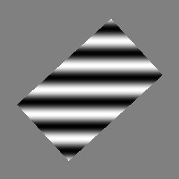
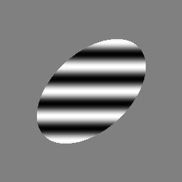
| Examples of envelopes with grating carriers | |
|---|---|
Stimulus generated by applying a hard-edge rotated square envelope with an aspect-ratio higher than 1 to produce its rectangular shape. |
Stimulus generated by applying a hard-edge rotated circular envelope with an aspect-ratio higher than 1 to produce its elliptic shape. |
Stimulus generated by applying a Gaussian rotated circular envelope with an aspect-ratio higher than 1 to produce its elliptic shape. |
Stimulus generated by applying a rotated circular envelope with an aspect-ratio higher than 1 to produce its elliptic shape. Note that a Gaussian modulation has been applied to the border of the envelope (ie: both size and sigma parameters have been set to a value different from 0). |
Note: You may refer to the following tutorials as they use Grating-like Stimuli in actual experiments: Contrast Sensitivity, Orientation Discrimination.
Checkerboard stimuli consist of Cartesian or polar 2D patterns with alternating and repetitive light and dark patches. They can be either contrast-defined or luminance-defined.
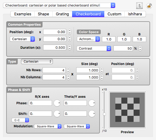
Cartesian type:
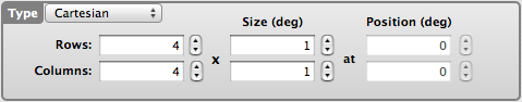
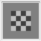
The number of rows and columns as well as the size for each of these in degree are specified here. Note that position is not used for the Cartesian type.
Polar type:
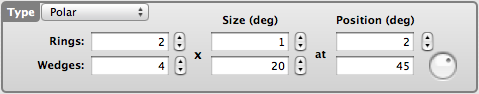
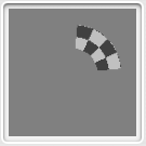
The number of rings and wedges as well as the size for each of these in degree are specified here. Position is used to shift the pattern along the radial direction (thus creating an annulus) and the angular direction (thus applying a rotation to the pattern).
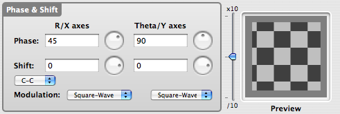
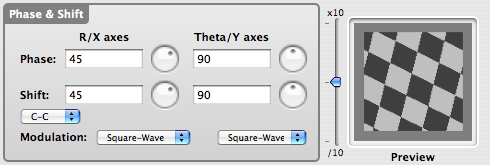
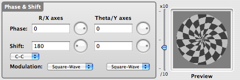
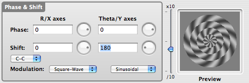
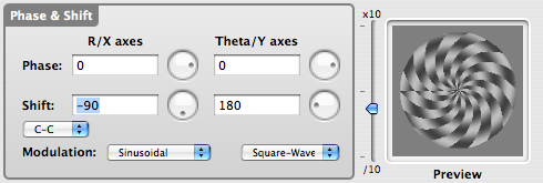
Parameters:
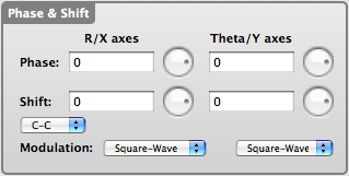
The parameters for checkerboard stimuli are:
the phase in deg along each stimulus dimension: (x,y) for Cartesian, (r, theta) for polar
the shift in one direction as a function of the other direction: the continuous or discrete nature of this shift is set through the associated pop-up menu (C-C for continuous shift along both dimensions; C-D for continuous along the r,x axes and discrete along the y,theta axes; D-C for discrete along the r,x axes and continuous along the y,theta axes; D-D for discrete shift along both dimensions)
the modulation profile (square-wave or sinusoidal)
Examples:
Note: You may refer to the tutorial Creating Retinotopic Mapping Stimuli as it heavily uses Checkerboard-like Stimuli animated over time.
Custom stimuli are computed from the evaluation of a sequence of mathematical expressions. Virtually any stimuli that can be described analytically in 2D, either by Cartesian or polar coordinates, can be generated using Psykinematix. They can be either contrast-defined or luminance-defined.
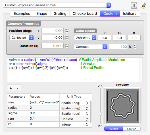
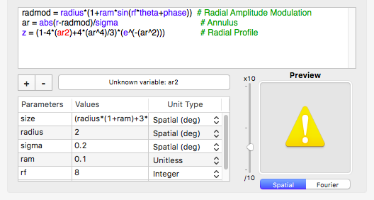
Expression Box:
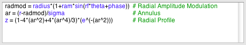
The analytical description of your custom stimuli should be entered and edited in the expression box. Reserved keywords (built-in constants, functions, and variables) are always displayed in blue while comments (starting with the # symbol) are in green. When the expressions contain a syntax error, the text background switches to red to indicate the problem, and automatically changes back to white once the problem is fixed. Unknown variables or functions are highlighted in red as well. When the expression cannot be evaluated because of evaluation errors (eg, "divide by zero"), the preview is replaced by a warning sign and a message is displayed above the expression with the source of the error:
Single line or multi-line assignment expressions can be used to describe how the stimulus is computed. Assignments on the same line should be separated by a semicolon and may be followed by a comment. Each assignment operation should follow the syntax:
<variable> = <expression>
with the last assignment being:
z = <expression> or zr = <expression>; zg = <expression>; zb = <expression>
or/and za = <expression>
where:
There are reserved variables that are unique to the expression box for custom stimuli:
| x, y | Cartesian coordinates | |
| r, theta | polar coordinates | |
| time | time relative to stimulus onset |
The predefined spatial variables x, y, r and theta are 2D arrays describing coordinates for each pixel of the stimulus.
Note that all variables used as operands in the expression box should be either a temporary user-defined variable, one of the above reserved variables, or one of the parameters defined in the Parameter Table (see below). Dependent and independent variables of experimental design should never be directly used in the expression box, however they could be used to specify the values of the parameters defined in the Parameter Table.
There are also reserved operations that are unique to the expression box for custom stimuli. These functions only applies on 2D arrays:
| Matrix operations: | ||
| shift(x,u,v) | Shift array x by u spatial units horizontally, and v spatial units vertically with wrapping and subpixel resolution through bilinear interpolation | |
| dshiftp(x,d) | Shift array x horizontally by array d on a pixel by pixel basis with subpixel resolution (positive shift only!) This function can be used to apply positive and negative disparity in stereo-pair stimuli | |
| conv(x,y) | 2D Convolution of x and y (done in Fourier space) | |
| norm(x,m,u) | Normalization of x so its mean is m and its maximum value is u | |
| scale(x,a,b) | Scale x between a and b | |
| mag(x) | Fourier magnitude of array x | |
| phase(x) | Fourier phase of array x | |
| ifft(m,p) | Inverse Fourier transform for magnitude array m and phase array p | Matrix to Scalar operations: |
| min(x) | Minimum value of matrix x | |
| max(x) | Maximum value of matrix x | |
| mean(x) | Mean value of matrix x | |
| std(x) | Standard deviation value of matrix x | |
| sum(x) | Sum value of matrix x | |
| length(x) | Length of matrix x (n^2 for a n x n matrix) | Special functions: |
| unoise(x,s,g) | 2D uniform noise between -1 and 1 with seed s (as integer), granularity g (in pixels) and the same size as x | |
| gnoise(x,m,u,s,g) | 2D Gaussian noise with mean m, std u, seed s (as integer), granularity g (in pixels) and the same size as x | |
| pnoise(x,y) | 2D Perlin noise at coordinate x,y with same size as x and y (fractal or pink noise can be created by rescaling Perlin noise and added into itself) | |
| bessj0(x) | 2D Bessel function of order 0 | |
| bessj1(x) | 2D Bessel function of order 1 | |
| bessjn(x,n) | 2D Bessel function of order n |
Note that all operations and functions used in the expression box are applied on a pixel basis when at least one of the operands consists of a 2D array. If the evaluation of the right part of an assignment results in a 2D array, the assigned temporary variable is internally represented as a 2D array as well; otherwise, it is simply represented as a scalar.
Although the evaluation of the expressions is highly optimized, typically several times faster than its Matlab® equivalent, here are few tips to further improve the evaluation performance for complex expressions:
The use of temporary variables is particularly helpful when the same sub-expression is reused several times in the evaluation.
However, do not overuse temporary variables as they may take a significant amount of memory if representing 2D arrays.
Instead use the built-in grating or checkerboard-based stimuli if appropriate as their generation is even more optimized in terms of speed and memory footage.
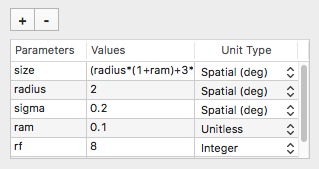
Parameters in this table are locally defined (ie: not available from outside the generation of the custom stimulus), and are used to specify some basic aspects of the custom stimulus. Their values are either fixed or under the control of an experimental method (dependent variables), subject specific variables, or independent variables. In addition to the parameters' names and values, their unit type should also be specified so their values get properly converted (eg: to pixel units if they represent spatial dimensions of the stimulus, or from degree units to radian units if they represent angular dimensions, see the table below for more details). Note that only these locally defined parameters can appear as operands in the expressions box.
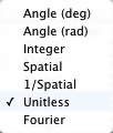 |
Unitless: | This unit expresses any amount that does not require any conversion and that is not affected by the geometry calibration data (default unit when adding a new parameter). |
| Integer: | This unit expresses an integer value either negative or positive. If the provided value is real, then it is converted to an integer by discarding the fractional part (ie: the value is truncated toward zero). | |
| Spatial (deg): | This unit expresses distance or angle of the visual field in degrees. It should be used in particular when manipulating the polar coordinate r or Cartesian coordinates x and y. The value is automatically converted to pixels with subpixel resolution for rendering purpose by using the geometry calibration data. | |
| Spatial (arcmin): | This unit expresses distance or angle of the visual field in minutes of arc (1/60 of one degree). It should be used in particular when creating stereo stimuli. The value is automatically converted to pixels with subpixel resolution for rendering purpose by using the geometry calibration data. | |
| Angle (deg): | This unit expresses an orientation angle in degrees. It should be used in particular when manipulating the polar coordinate theta. The value is automatically converted to radians before use. | |
| Angle (rad): | This unit expresses an orientation angle in radians. It should be used in particular when manipulating the polar coordinate theta. | |
| 1/Spatial (cpd): | This unit expresses the reciprocal of the distance or angle of the visual field in cycles per degree. It should be used in particular when manipulating the polar coordinate r or Cartesian coordinates x and y to express spatial frequency. The value is automatically converted to cycles per pixel for rendering purpose by using the geometry calibration data. | |
| Fourier: | This unit expresses spatial frequency in cycles per degree when expressing visual stimuli in the Fourier domain and using the ifft function (inverse Fourier transform). Note that parameters with the Fourier unit should not be used to specify the size parameter (see below). | |
| Image File: | Not an unit per se, but a convenient way to import an image file as a 2D variable that can be manipulated through convolution, Fourier transform, or direct access to the chromatic components. Each chromatic component is stored as a variable with the 'r', 'g', 'b' and 'a' suffixes added to its name (eg: if the variable is named 'image' then its red, green, blue and alpha components are accessible using the 'imager', 'imageg', 'imageb' and 'imagea' variables, respectively). The imported images are automatically scaled to the 'size' parameter (see below). |
A parameter 'size' is present by default in the Parameter Table. This parameter specifies the spatial extent in degree of visual angle for the square texture representation of the stimulus in the video memory. This allows the stimulus generation to be restricted to the useful area covered by the stimulus rather than over the whole display. The value for the 'size' parameter can itself be an expression (without the = assignment) based on the other parameters. For example, if an annulus stimulus is parameterized with 'radius' and 'sigma' parameters, a size of '2*(radius+2*sigma)' for the generated texture will closely match the useful area covered by the stimulus. The boundaries of the area delimited by the 'size' parameter are represented by a black frame around the stimulus preview (zoom out if the surrounding frame does not show up).
Note that the evaluation of the other parameters should not depend on any parameters present in the table; otherwise, their evaluation results may be undefined. On the contrary, the evaluation of 'size' should depend on the parameters present in the table only (with the exception of the parameters in Fourier unit) and not on the experiment variables.
Examples:
z = cos(x/5)
|
z = cos(x/5)*sin(y/5)
|
z = cos(x/5+sin(y/10))
|
z = sin(r/5)
|
z = cos(theta*10)
|
z = sin(r/5)*cos(theta*10)
|
z = cos(r+theta)
|
z = cos(r+theta*10)
|
z = cos(r/5+theta*10)
|
z = cos(x/5)+cos(r)
|
z = sin(1000/(r+20))
|
z = sin(exp(r/20))*cos(theta*10)
|
z = e^(-(r^2)/1000)
|
z = cos(x/5)*e^(-(r^2)/1000)
|
z = unoise(x,irand,8)
|
Note: You may refer to the tutorial Creating Filtered Noise Stimuli as it heavily uses Custom Stimuli.
Ishihara-like stimuli are disk-sampled shapes that are commonly used to test color vision in the clinic (for example Ishihara pseudoisochromatic plates for screening red-green colour vision deficiency or the Cambridge Colour Test). Ishihara stimuli consist typically in a target shape differing in chromaticity from the background. The target and background are made up of many discrete discs within their own boundary and the luminances of the individual discs are randomized to ensure that the subject detects the target only by true color vision without relying on edge artifacts or luminance differences. However Ishihara-like stimuli can also be used to investigate figure-ground segregation in general.
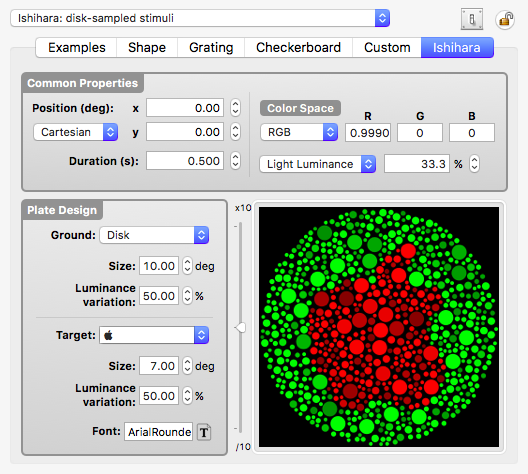
The chromaticities of the target and ground can be defined separately in the common properties section using the "Light Luminance" option for the figure chromaticity and the "Dark Luminance" option for the ground chromaticity.
The Plate Design section defines other properties: the shape and size of both background and target. Luminance variation can be added to each component as well. Shape of the background can be either a disk or a square (size refers to diameter or side respectively), and the target can be of different shapes:
For the Landolt-C and Tumbling-E optotypes the stroke width is 1/5 of the size, and the gap in the Landolt-C has the same width as its stroke. The orientation of these 2 optotypes can be changed by specifying a value (or a random variable) for its 'Rendering' orientation in the Control Settings palette. The appearance of all other targets (digits, optotypes and custom symbols) is defined by the selected font, but their size depends on the specified target size in degree and not on the font size.
Note that the system-defined variable [SELECTION] always contains the randomly selected target so the subject's response can be checked in a discrimination procedure for example.
Committee on Vision, Assembly of Behavioral and Social Sciences, National Research Council (1981) Procedures for Testing Color Vision: Report of Working Group 41. National Academy Press: Washington, D.C. (PDF)
Mollon, J.D. and Regan, B.C. (2000) Cambridge Colour Test Handbook (PDF)
Smith V.C., Pokorny J. (2003) Color Matching and Color Discrimination. The Science of Color edited by Steven K. Shevell, 2nd Edition (PDF)
© 2006-2024 KyberVision Japan LLC. All rights reserved.
Matlab is a registered trademark of The MathWorks, Inc.


.png)
*sin(y%3A5).png)
).png)
.png)
.png)
*cos(theta*10).png)
.png)
.png)
.png)
+cos(r).png)
).png)
)*cos(theta*10).png)
%3A1000).png)
*e%5E(-(r%5E2)%3A1000).png)
.png)